Modelling of running
performance and training
Modélisation de l’entraînement et de la performance en course à pied
Franck Tancret
e-mail:
franck.tancret@polytech.univ-nantes.fr
ABSTRACT
The influence of
training parameters on the performances of a male middle-distance runner has
been quantitatively modelled by a Gaussian processes statistical regression
software. The latter produces a non-linear multi-dimensional regression model
of the running performance as a function of relevant training parameters. The
database was constituted of the athlete’s actual training schedules and race
performances over several outdoor track seasons on 800 m, 1000 m and
1500 m. The respective effects and interactions of the three main kinds of
training sessions have been identified (endurance, resistance, and sprint), and
succesfully compared to commonly accepted qualitative trends. The model is able to predict the performances of an athlete
given a complete season’s training record, and can subsequently be used by the
coach to optimise the training schedule and race performance.
INTRODUCTION
Understanding and
modelling athletic training and performance is a very tricky task that has
generated lots of scientific work in many various fields such as medecine,
physiology (Billat, 1996; Craig et al.,
1993; Di Prampero et al., 1998;
Fukuba et al., 1993; Green and
Dawson, 1993; Hausswirth and Brisswalter, 1999), nutrition (Tsintzas and
Williams, 1998), biomechanics (Anderson, 1996; Morgan et al., 1994; Novacheck, 1996; Nummela et al., 1996), psychology (Crews, 1992), statistics (Grubb, 1998;
Léger and Mercier, 1984), etc... Moreover, most of the performance prediction
studies consist in establishing relations between the present physiological or
physical characteristics of athletes and their expected performance in a near
future (Babineau and Léger, 1997; Bannister and Fitzclarke, 1993).
Nevertheless, the relation between training and performance is so complex that
only separate aspects are clearly scientifically understood, and require often
time-demanding and expensive experiments. Moreover, in order to identify
precisely the role of each individual parameter, those tests are almost always
carried out in very precise conditions which do not necessarily reflect the
context of an athlete’s normal life. As a consequence, even if of capital
qualitative importance for coaches, the results usually cannot be simply applied
to optimise the training schedule of individual athletes, and only a few
attempts on global modelling have been performed (Morton, 1997).
In this
work, a preliminary study is carried out to model directly, and as a whole, the
effect of training parameters during a complete season on the performance of a
given athlete. More precisely, the influence of the three main kinds of sessions
(endurance, resistance, and sprint) on the race performance of a
middle-distance runner (800 m to 1500 m) has been modelled using a
Gaussian processes software. Gaussian processes are able to perform a kind of
non-linear, multiparametric regression of one output —in this case the athletic
performance— as a function of many different input parameters —here the amount
of training in different effort categories, the advancement of the season, the
number of races run, etc... They can then be used to predict the output value,
i.e. athletic performance, given a set of new inputs —a new training schedule.
GAUSSIAN
PROCESSES MODELLING
If you do not feel comfortable with statistical theories and, more generally, with mathematics, you can easily skip this section!
Although already
documented in the literature (Gibbs, 1998; Williams and Rasmussen, 1996), but because
they are the basic modelling tool of the present study, Gaussian processes
should be first briefly presented.
Let’s consider
the data, D, as a set of N L-dimensional
input vectors {x1, x2,..., xN} = [XN]
and their corresponding outputs, or targets, {t1, t2,..., tN} = tN.
In the present case the L dimensions
will correspond to the L training
parameters supposed to have an influence on athletic performance. Each of the N inputs will correspond to the training
history before each of the N race performances
(outputs) used to create the model. Now, if one wants to predict the athletic
performance that can be expected with a new training schedule, it is necessary
to calculate the output, tN+1,
corresponding to a new input vector, xN+1.
The joint probability
distribution, in an N-dimensional
space, of the N output values in the
database given the N input vectors,
is P(tNï[XN] ). In a similar way, the joint
probability distribution of the N
data points plus the single new point with input vector xN+1,
for which we want to predict the output tN+1,
is P(tN+1, tNçxN+1, [XN]). We are looking
for the one-dimensional probability distribution over the predicted point, P(tN+1çxN+1, D}, given the
corresponding input vector, xN+1,
and the data D = { tN, [XN] }.
A relationship exists between the above quantities (Gibbs, 1998):
![]() (1)
(1)
We define this
distribution as a Gaussian process (GP), in assuming that the joint probability
distribution of any N output values is
a multivariate Gaussian,
![]() (2)
(2)
where µ
is the mean, [CN] a
covariance matrix which is a function of [XN],
and Q a set of
parameters which will be discussed later. Consequently, a similar equation
—with N+1 variables— holds for ![]() , and equation (1) reduces to a univariate Gaussian (Gibbs,
1998):
, and equation (1) reduces to a univariate Gaussian (Gibbs,
1998):

![]() (3)
(3)
where ![]() is the posterior mean
(i.e. the value of the predicted output) and
is the posterior mean
(i.e. the value of the predicted output) and ![]() the standard
deviation (i.e. an indication of the prediction error):
the standard
deviation (i.e. an indication of the prediction error):
![]() and
and ![]() (4)(5)
(4)(5)
where
![]() and
and ![]() (6)(7)
(6)(7)
Equation (3) gives
the probability distribution of the new output, tN+1, given the new input vector, xN+1,
and the data, D. The mean prediction,
![]() , and its standard deviation,
, and its standard deviation, ![]() , depend on the covariance matrix, [CN], which elements Cij
are given by the covariance function, C.
This function is extremely important because it embodies our assumptions about
the nature of the underlying input-output function we want to model. In other
words, it defines how strongly any input will influence the value of the
output. The covariance function used in the present work is
, depend on the covariance matrix, [CN], which elements Cij
are given by the covariance function, C.
This function is extremely important because it embodies our assumptions about
the nature of the underlying input-output function we want to model. In other
words, it defines how strongly any input will influence the value of the
output. The covariance function used in the present work is
 (8)
(8)
where Q = {![]() (l = 1 to L), q1, q2, sn}.
(l = 1 to L), q1, q2, sn}.
This function
gives the covariance between any two outputs, ti and tj,
with corresponding input vectors xi and xj.
The closer the inputs, the smaller the exponent in the first term of equation
(8), the larger the first term, and the stronger the outputs will be correlated,
making it probable that they have close values. This first term also includes
the length scales, ![]() , over which the function will be able to vary in any of the L input dimensions.
, over which the function will be able to vary in any of the L input dimensions. ![]() indicates the smoothness of the interpolant in the
indicates the smoothness of the interpolant in the ![]() th dimension: no
long-range correlations in the data on lengthscales much bigger than
th dimension: no
long-range correlations in the data on lengthscales much bigger than ![]() are to be expected.
are to be expected.
The second term, q2, is an offset,
allowing the functions to have a non-zero mean value. The last term, ![]() , is the noise model, with dij being equal to 1
if i = j and to 0
otherwise. We have thus an input-independent noise model of variance
, is the noise model, with dij being equal to 1
if i = j and to 0
otherwise. We have thus an input-independent noise model of variance ![]() for the output, and
we are assuming the inputs to be noise-free. In the present case, the “noise”
in the outputs can be due to race conditions —weather, global level of the
race, tactics— or to different health or psychological state of the athlete
from race to race.
for the output, and
we are assuming the inputs to be noise-free. In the present case, the “noise”
in the outputs can be due to race conditions —weather, global level of the
race, tactics— or to different health or psychological state of the athlete
from race to race.
The parameters Q = {![]() (l = 1 to L), q1, q2, sn} are called hyperparameters
because they define the probability distribution over functions rather than the
interpolating function itself. These hyperparameters, Q, the dataset, [XN], tN,
and the new input vector, xN+1, define completely the
value of the prediction, or output,
(l = 1 to L), q1, q2, sn} are called hyperparameters
because they define the probability distribution over functions rather than the
interpolating function itself. These hyperparameters, Q, the dataset, [XN], tN,
and the new input vector, xN+1, define completely the
value of the prediction, or output, ![]() , and of its standard deviation,
, and of its standard deviation, ![]() . The optimum values of the hyperparameters are inferred by
the computer software during the training of the model by maximizing the
probability of the hyperparameters given the data, P(QçD), which is done numerically within a Bayesian
framework (Gibbs, 1998).
. The optimum values of the hyperparameters are inferred by
the computer software during the training of the model by maximizing the
probability of the hyperparameters given the data, P(QçD), which is done numerically within a Bayesian
framework (Gibbs, 1998).
In the present
problem, a Gaussian processes model has been optimised in order to predict what
performance (![]() ) can be expected from a particular athlete given his whole
training record ( [XN] )
and race performances (tN) over several seasons. The
advantage of this kind of modelling is that it doesn’t need any knowledge about
the scientific parameters that influence performance, and it is able to take
all the interactions between training parameters into account. However, before
making any prediction, it is of technical interest to check if the model is
able to reproduce well-know training trends, such as the individual effect of
endurance, resistance, sprint, etc., on the race performance.
) can be expected from a particular athlete given his whole
training record ( [XN] )
and race performances (tN) over several seasons. The
advantage of this kind of modelling is that it doesn’t need any knowledge about
the scientific parameters that influence performance, and it is able to take
all the interactions between training parameters into account. However, before
making any prediction, it is of technical interest to check if the model is
able to reproduce well-know training trends, such as the individual effect of
endurance, resistance, sprint, etc., on the race performance.
THE DATABASE
The database has
been constituted from the training and race records of 6 spring/summer seasons
of a unique male middle-distance runner, between 21 and 26 years old, with
personal bests of 1 min 56.3 s (116.3 s) on 800 m and
3 min 58.8 s (238.8 s) on 1500 m, achieved at the age
of 22 and 26, respectively. In all cases, the spring/summer outdoor seasons
started at the end of March or beginning of April, following a period of 2 to 4
weeks of relative rest (two or three 30 to 45 minute steady jogs a week) after
either a cross-country winter season or a coupled cross-country and indoor
track season on 800 m / 1500 m. Consequently, the first two parameters
are the age and a boolean input indicating the nature of the winter season
(cross-country, or cross-country and indoor track), since this is likely to
modify the endurance, resistance and/or speed background of the athlete at the
beginning of the outdoor track season.
As this work
represents a preliminary study, the problem has been voluntarily
oversimplified, and only a few training parameters, supposedly of main
importance, have been taken into account: the number of three different kinds
of training sessions thereafter called endurance, resistance, and sprint
(defined and discussed later), and the number of training weeks and of races
run since the beginning of the outdoor track season. The output, i.e. race
performance on 800 m, 1000 m or 1500 m, is given by the
Hungarian Scoring Table. All the parameters, as long as their minimum and
maximum values in the database, are presented in Table 1. The database was
constituted of 30 lines, i.e. race results.
|
Parameter |
Minimum |
Maximum |
Comments |
|
Age |
21 |
26 |
in years |
|
Type of winter
season |
0 |
1 |
0 =
cross-country 1 =
cross-country + indoor track |
|
Number of weeks
since start of season |
3.143 |
17 |
|
|
Number of
endurance sessions since start of season |
5 |
30 |
|
|
Number of resistance
sessions since start of season |
4 |
36 |
|
|
Number of
sprint sessions since start of season |
1 |
14 |
|
|
Number of races
since start of season |
0 |
9 |
|
|
Output:
performance |
689 |
868 |
in points for 800, 1000 or
1500 m |
Table 1: input and output parameters in the database, and their extremum values
The concepts of
endurance, resistance, and sprint sessions considered in this study must be
explicited:
- Endurance:
easy steady-state running sessions of typically 30 to 45 minutes used to
develop endurance, as well as regeneration sessions (Hawley et al., 1997).
- Resistance:
refers to a quite wide range of sessions, usually done on the track, and
constituted of repetitions of fractions mainly from 100 m to 500 m,
run at paces close to 800 m or 1500 m races, with a cumulated length
most often comprised between 1200 m and 2000 m. The rest between
fractions can be made jogging or walking, and last between one and three times
the duration of the previous fraction. A wide range of different sessions are
included in this category, for example the so-called “interval-training”, but
they all have the common goal of improving the basic resistance at race pace.
Even if still discussed scientifically (Keith et al., 1992), they are commonly accepted as one of the main
factors to improve performance (Hawley et
al., 1997; Lindsay et al., 1996;
Tanaka and Swensen, 1998), and often represent 50% or more of the number of
sessions in middle-distance training.
- Sprint,
or speed: these sessions aim to develop the basic speed, which is also believed
to be a relevant factor (Jensen et al.,
1997). These sessions usually consist in repetitions of fractions of 40 m
to 150 m, run at full speed, with a walking rest until “complete”
recovery, for a cumulative length mostly comprised between 400 m and
800 m.
It should be
noted that all these parameters are very simple to characterise, but that each
of them implies many complex physiological and biomechanical phenomena, none of
them being completely scientifically understood. As a consequence, the chosen
parameters do not represent the real
basic parameters of running. However, and that is the main purpose of the
present study, they represent a very practical basis for the design of new
training schedules, because they are coaching parameters.
Moreover, as this
is only a preliminary study, no information about the actual content of each
session has been included. This point will be discussed later.
MODELLING AND RESULTS
1 -
Modelling
The “Tpros”* Gaussian processes software, developed
by the University of Cambridge, UK, has been used to create the inputs-output
fit. A good indicator of the effectiveness of the modelling is the comparison
of predicted versus actual outputs for the inputs contained in the database.
This is plotted in figure 1, where it can be seen that a rather good agreement
between actual performance and predictions is obtained. This is the first indicator
of a good model. It should be reminded that error bars, as calculated from
equations (5) and (8), contain both a predictive uncertainty and an estimation
of the noise in the database.

Figure 1: Comparison between actual and predicted race performances for the inputs of the database.
2 -
Testing trends
The ability of
the model to reproduce values of the output that have been used to train it is
not sufficient, because this does not tell if the model is able to generalise
well, i.e. to make reliable predictions in unknown cases. Thus, to better
assess the validity of the model, it is interesting to check if it is able to
reproduce practically well-known or scientifically understood training trends.
It is not here
the purpose to test extensively and systematically all possible trends, but to
give a few examples to show how the model is able to deal with raw data.
First, since
resistance training is supposed to be of major importance, its substitution to
either endurance or sprint training has been investigated. Figure 2 show the
influence of the number of resistance sessions on race performance for a
constant number of ‘resistance + endurance’ sessions (39), all other parameters
being fixed (cross-country winter season, age 26, 12th week of the
season, 6 sprint sessions and 6 races run). It is clear that replacing
endurance training by resistance training improves performance. However, it is
worth reminding that abusing of this kind of substitution may cause
overtraining, fatigue, and injuries: even if the actual trend is correctly
predicted, it is the duty of the coach to interpret and adjust results to the
athlete’s training schedule.

Figure 2: Evolution of the predicted performance when endurance training is replaced by resistance training.
As the number of resistance sessions increases, that of endurance sessions decreases equally.
Dashed lines: error bounds.
Similarly, figure
3 shows the effect of replacing sprint training by resistance, all other parameters
kept constant (cross-country winter season, age 21, 15th week of the
season, 24 endurance sessions and 6 races run). Once more, increasing the
proportion of resistance globally increases race performance, but it is
interesting to note that the curve reaches a plateau: if sprint is almost
suppressed, there is finally a lack of basic speed which prevents the athlete
from improving further, especially on short distances (e.g. 800 m), which
is well known by all coaches.

Figure 3: Evolution of the predicted performance when sprint training is replaced by resistance training.
As the number of resistance sessions increases, that of sprint sessions decreases equally.
Dashed lines: error bounds.
The second set of
tested trends concerns the effect of an increase in training, by adding either
endurance or resistance sessions, all other parameters being fixed
(cross-country winter season, age 24, 12th week of the season, 6
sprint sessions and 6 races run).
Figure 4 shows
that increasing the number of endurance sessions alone has almost no effect on
race performance. It is known that endurance does not directly improve
middle-distance running performance —so that the model predictions are
correct—, but it is also kown that it is necessary for injury-free long-lasting
seasons and for general recovery —which is ignored by the model.
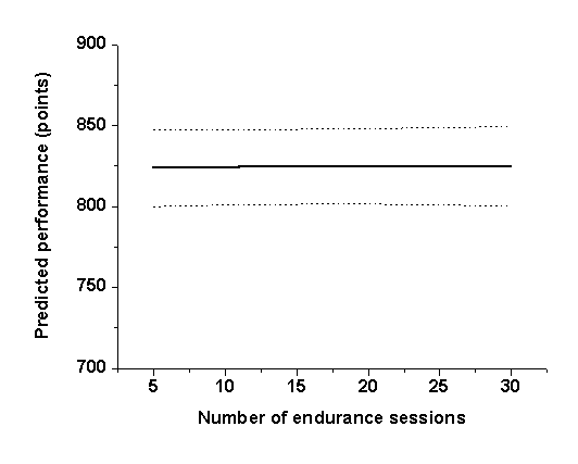
Figure 4: Predicted performance when the number of endurance sessions increases. Dashed lines: error bounds.
Finally, figure 5
shows a significant positive effect of increasing the number of resistance
sessions on race performance, which is also consistent with basic coaching
knowledge. Once more, if this type of sessions is repeated too often, this can
yield overtraining and injuries, but this is not known by the model since the
data concerned only “normal” training.

Figure 5: Predicted performance when the number of resistance sessions increases. Dashed lines: error bounds.
3 -
Making predictions
Only
once tested, the model can be trusted to make performance predictions for new
training schedules, and to try and optimise training prameters to improve
performance. In this aim, predictions were made in varying slightly the training
schedule parameters from the two best performances of the database.
For example, one of those best performances was achieved after an indoor track season, the other one after a cross-country winter season. In the former case, changing the nature of the winter season from indoor to cross-country decreases the race perfomance by 14.6 points, i.e. a loss of 0.63 seconds on 800 m or 1.27 seconds on 1500 m. In the second case, changing from cross-country to indoor increases the perfomance by 10.1 points, i.e. a gain of 0.44 seconds on 800 m or 0.89 seconds on 1500 m. In both cases, this indicates the beneficial effect on an indoor track winter season on the outdoor track summer performance. This can be understood by a gain in initial resistance and speed at the beginning of the summer season. Even if this could seem obvious for most coaches, there was so far no strict evidence.
The ‘Tpros’
software is able to find extrema in the output by input optimisation. This has
been made to maximise performance, starting from the inputs corresponding to the
two best performances, and setting the winter season as indoor track and the
age as 26. Inputs converged to similar values in both cases. Inputs for session
numbers have then been set to the closest integer value, and a new prediction
has been performed with the obtained following inputs: 15 weeks and 7 races run
since start of outdoor track season, 23, 34 and 5 endurance, resistance and
sprint sessions, respectively. This led to an increase of 17 and 35 points with
respect to the two best predicted performances for inputs of the database,
corresponding respectively to a gain of 0.73 s and 1.51 s on
800 m, or of 1.49 s and 3.06 s on 1500 m. If confirmed by
actual experiment, such improvements could make the difference for a
qualification, a victory, or a personal record.
CONCLUSIONS AND PERSPECTIVES
A Gaussian
processes regression computer software has been used to model and predict the
athletic performances of a male middle-distance runner (800 m to
1500 m), as a function of various simplified components of his training
records over a complete season: respective amounts of endurance, resistance,
and sprint, advancement of the season... The model is able to reproduce
successfully the influence of various training trends in a given context, as
well as interactions between them: effects of increasing the amount of
endurance or resistance, substituting endurance or sprint by resistance, etc...
It can
thus be used to predict the possible performances of an athlete given his
season’s training programme only, and, to some extent, to design a new training
schedule to increase performance. However, since the parameters used in this
study have been voluntarily oversimplified —e.g. “resistance” holds for any
kind of session with repetitions run close to race pace— the present study
constitutes only a preliminary but promising work in the field of training
modelling. Indeed, it could be possible in the future to include other
parameters, allowing for example a more precise description of “resistance”
sessions: number of repetitions, length and speed, recovery between
repetitions, total distance... Nevertheless, it should be kept in mind that
including too many parameters may lead to modelling uncertainties, in
particular if the range of values encountered for each input is too small.
Consequently, it might be useful to limit the description of resistance
sessions to a kind of “equivalent work charge”, the latter needing to be
otherwise defined. Also, the present model did not take into account any
indication of overtraining (which was obviously absent in the present case),
nor tapers, which are important factors influencing race performance (Bannister
et al., 1999; Mujika, 1998; Shepley et al., 1992).
At a more
ambitious scale, this kind of approach could be extended to a “universal”
training model, taking into account the training records and performances of
many different athletes. For this, it should be necessary to “normalise” the
performances of all the athletes (for example by their personal best), and,
possibly, to take other personal characteristics into account, so that the
results can be applied to any athlete. Given the previously exposed
possibilities of such a modelling approach, it is obvious that further research
has to be done in this area.
Finally, it must
be kept in mind that the present approach is purely empirical, and includes
implicitely —through the design of training sessions itself— results from
decades of training science. Consequently, it does not constitute a replacement
for training science and theory, which are still needed in the long term to
better understand the fundamental mechanisms of exercise, and to improve
training sessions themselves. Nevertheless, the present approach could be a
very powerful tool for coaches in the short term.
ACKNOWLEDGMENTS
The author would
like to thank Mr. Jacky Wattebled (Comité Omnisports de la Bresle, Eu, France)
and Mr. Dominique Pignet (Stade Malherbe Athletic Caennais, Caen, France) for
their technical advice within the Fédération Française d’Athlétisme.
REFERENCES
Anderson,
T. (1996). Biomechanics and running economy. Sports Medicine, 22(2),
76-89.
Babineau,
C. and Léger, L. (1997). Physiological response of 5/1 intermittent aerobic
exercise and its relationship to 5km endurance performance. International Journal of Sports Medicine,
18(1), 13-19.
Bannister,
E.W. and Fitzclarke, J.R. (1993). Plasticity of response to equal quantities of
endurance training separated by non-training in humans. Journal of Thermal Biology, 18(5-6),
587-597.
Bannister,
E.W., Carter, J.B. and Zardakas, P.C. (1999). Training theory and taper:
validation in triathlon athletes. European
Journal of Applied Physiology and Occupational Physiology, 79(2), 182-191.
Billat,
L.V. (1996). Use of blood lactate measurements for prediction of exercise
performance and for control of training - Recommandations for long-distance
running. Sports Medicine, 22(3), 157-175.
Craig,
N.P., Norton, K.I., Bourdon, P.C., Woolford, S.M., Stanef, T., Squires, B.,
Olds, T.S., Conyers, R.A.J. and Walsh, C.B.V. (1993). Aerobic and anaerobic
indexes contributing to track endurance cycling performance. European Journal of Applied Physiology and
Occupational Physiology, 67(2),
150-158.
Crews,
D.J.(1992). Psychological state and running economy. Medicine and Science in Sports and Exercise, 24(4), 475-482.
Di
Prampero, P.E., Fusi, S. and Antonutto, G. (1998). The concept of lactate
threshold. A critical review. Medicina
dello Sport, 51(4), 393-400.
Fukuba,
Y., Walsh, M.L., Cameron, B.J., Morton, R.H., Kenny, C.T.C. and Bannister E.W.
(1993). Lactate modeling and its application to endurance training. Journal of Thermal Biology, 18(5-6), 617-622.
Gibbs, M.N. (1998). Bayesian Gaussian proceses for
regression and classification. PhD Thesis, University of Cambridge, UK.
Green,
S. and Dawson, B. (1993). Measurement of anaerobic capacities in humans -
Definitions, limitations and unsolved problems. Sports Medicine, 15(5),
312-327.
Grubb,
H.J. (1998). Model for comparing athletic performances. The Statistician, 47(3),
509-521.
Hausswirth,
C. and Brisswalter, J. (1999). Factors modifying running economy in long
distance running. Science & Sports,
14(2), 59-70.
Hawley,
J.A., Myburgh, K.H., Noakes, T.D. and Dennis, S.C. (1997). Training techniques
to improve fatigue resistance and enhance endurance performance. Journal of Sports Sciences, 15(3), 325-333.
Jensen,
J., Jacobsen, S.T., Hetland, S. and Tveit, P. (1997). Effect of combined
endurance, strength and sprint training on maximal oxygen uptake, isometric
strength and sprint performance in female elite handball players during a
season. International Journal of Sports
Medicine, 18(5), 354-358.
Keith,
S.P., Jacobs, I. and McLellan, T.M. (1992). Adaptations to training at the
individual anaerobic threshold. European
Journal of Applied Physiology and Occupational Physiology, 65(4), 316-323.
Léger,
L. and Mercier, D. (1984). Regressions in the VO2 max and running performance
(0.2 km to 42.2km). Journal
de Physiologie, 79(5), A80.
Lindsay, F.H., Hawley, J.A., Myburgh, K.H., Schomer, H.H., Noakes, T.D. and
Dennis, S.C. (1996). Improved athletic performance in highly trained
cyclists after interval training. Medicine
and Science in Sports and Exercise, 28(11),
1427-1434.
Morgan,
D., Martin, P., Craib, M., Caruso, C., Clifton, R. and Hopewell, R. (1994).
Effect of step length optimization on the aerobic demand of running. Journal of Applied Physiology, 77(1), 245-251.
Morton,
R.H. (1997). Modelling training and overtraining. Journal of Sports Sciences, 15(3),
335-340.
Mujika,
I. (1998). The influence of training characteristics and tapering on the
adaptation in highly trained individuals: A review. International Journal of Sports Medicine, 19(7), 439-446.
Novacheck,
T.F. (1996). The biomechanics of running. Gait
and Posture, 7(1), 77-95.
Nummela, A., StrayGundersen, J. and Rusko, H. (1996). Effects of
fatigue on stride characteristics during a short-term maximal run. Journal of Applied Biomechanics, 12(2), 151-160.
Shepley,
B., MacDougall, J.D., Cipriano, N., Sutton, J.R., Tarnopolsky, M.A. and Coates,
G. (1992). Physiological effects of tapering in highly trained athletes. Journal of Applied Physiology, 72(2), 706-711.
Tanaka,
H. and Swensen, T. (1998). Impact of resistance training on endurance
performance - A new form of cross-training?. Sports Medicine, 25(3),
191-200.
Tsintzas,
K. and Williams, C. (1998). Human muscle glycogen metabolism during exercise -
Effect of carbohydrate supplementation. Sports
Medicine, 25(1), 7-23.
Williams,
C.K.I. and Rasmussen, C.E. (1996). Gaussian processes for regression. In Advances in Neural Information Processing
Systems 8, MIT Press.